Mizuhashi Simple Domain

Lab no - 0x37, tired but here is another one, what was the mode again?, resistance, impedance, admittance, oh wait….

author: Vx

I spent 5 hours solving this one, just because I am EE student and seeing resistance, impedance, admittance makes me horny.

Ok lets start by decoding the description. At first glance I couldn’t understand anything.

I didn’t even new anything about the s3p file. (suscept.s3p)

I run some google searches and gpt and found out that s3p is used to store S-parameters of a 3-port network. (got scared, wtf is 3 port network, our syllabus has 2 port only)

Now without digging deeper into 3 port networks and what S-parameters actually are. I just searched for online how to view s3p files.

I got a code snippet using python scikit-rf library, that can plot the 3 port network parameters (S, z etc).

import skrf as rf

ntw = rf.Network('suscept.s3p')
ntw.plot_s_smith()

(In between this I also got to know that there are in total 9 S-parameters for a 3 port network for each frequency which is a 3x3 matrix, each S parameter is a complex number)

Well I got to know there are various plots for s parameters like magnitude(in dB) vs frequency, smith chart, phase vs frequency etc.

I plotted all of them one by one and checked the plots.

for example here is a smith chart for S-parameters s_smith

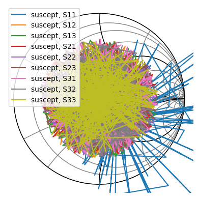
Idk anything about paramters what they actually mean, but I was sure that S11 is showing some abnormal behaviour compared to other parameters.

I confirmed in ticket from author, if it was parameter S11 that I need to focus on and he said YES!

So, I pointed all my eyes on S11 plots.

I have plotted various graphs for S11 parameter.

Like s11 magnitude(in dB) vs Frequency

s11 phase vs Frequency
s11 smith chart
s11 polar plot etc. etc.

But nothing made sense to me.

My initial thought was that maybe I need to get some hidden message out of the plot values of s11 magnitude or phase by applying some threshold to the values and then scale the remaining value in such a way that it form ascii values of flag characters. For once I thought 0x37 could be the scaling factor or some sort of offset.

To approve my theory, I did various experiments but nothing seems to work.

I felt like I am going in circles.

Progress back to 0.

Then I thought maybe I need to check the other parameters like impedance(z), admittance(y) or resistance(r).

Because they were given in challenge description.

I searched for formulas to convert s-parameters to z,y,r parameters.

For s11 parameter, the formulas are as follows:

Note -

How S paramters for a given frequency looks in a matrix -
[[S11 S12 S13]
 [S21 S22 S23
 [S31 S32 S33]]

# Impedance (Z), Admittance (Y), Resistance (R) from S11

Z11 = Z0 * ((1 + S11) / (1 - S11))

Y11 = (1 / Z0) * ((1 - S11) / (1 + S11))

R11 = Re(Z11)

Where Z0 is the characteristic impedance, usually 50 ohms (thanks to GPT).

I wrote a code to convert s11 to z11, y11, r11 using above formulas. Then I plotted the graphs for these parameters.

import numpy as np
import skrf as rf

ntw = rf.Network('suscept.s3p')

s11 = ntw.s[:,0,0]  # S11 parameter
Z0 = 50  # Characteristic impedance

z11 = Z0 * ((1 + s11) / (1 - s11))
y11 = (1 / z11)
r11 = np.real(z11)

Then i tried plotting z11, y11, r11 parameters wrt frequency.


import matplotlib.pyplot as plt

plt.figure(figsize=(12, 8))
plt.subplot(3, 1, 1)
plt.plot(ntw.f, np.abs(z11), label='|Z11|')
plt.title('Z11 Parameter')
plt.xlabel('Frequency (Hz)')
plt.ylabel('|Z11| (Ohms)')
plt.grid()

plt.subplot(3, 1, 2)
plt.plot(ntw.f, np.abs(y11), label='|Y11|', color='orange')
plt.title('Y11 Parameter')
plt.xlabel('Frequency (Hz)')
plt.ylabel('|Y11| (Siemens)')
plt.grid()

plt.subplot(3, 1, 3)
plt.plot(ntw.f, r11, label='R11', color='green')
plt.title('R11 Parameter')
plt.xlabel('Frequency (Hz)')
plt.ylabel('R11 (Ohms)')
plt.grid()

plt.show()

This shows the following plots: z11_y11_r11

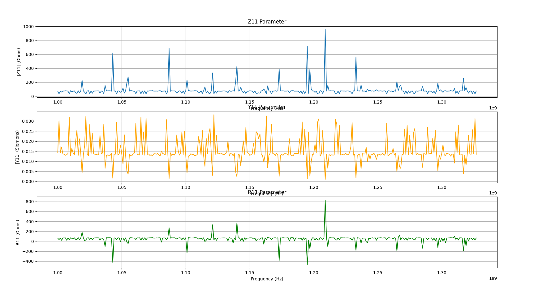
Umm strange I wasn’t able to find anything useful here.

Again nothing made sense to me. I got hopeless again.

Then I hopped again to tickets and this time I got something useful.

ticket1

The author said that there is no need to plot r11, y11 or z11 wrt frequency. Just plot them as it is.

This is a hint to plot the parameters in complex plane. Now my work got a little easy, as I know r11 is real value only, so I can ignore it.

All I need is to plot complex-plane (real vs img) for impedances(z11) and admittances (y11)

conductance = np.real(y11) # real part of admittance
susceptance = np.imag(y11) # imaginary part of admittance

resistance = np.real(z11) # real part of impedance
reactance = np.imag(z11) # imaginary part of impedance

fig, axs = plt.subplots(2, 1, figsize=(10, 15))

# Plot 1: Impedance (Real vs Imag)
axs[0].set_title('Impedance Complex Plane (Resistance vs Reactance)')
axs[0].set_xlabel('Resistance ($R$) [S]')
axs[0].set_ylabel('Reactance ($X$) [S]')
axs[0].plot(resistance, reactance, linestyle='None', marker='.', markersize=3, color='green')
axs[0].grid(True)


# Plot 2: Admittance (Real vs Imag)
axs[1].set_title('Admittance Complex Plane (Conductance vs Susceptance)')
axs[1].set_xlabel('Conductance ($G$) [S]')
axs[1].set_ylabel('Susceptance ($B$) [S]')
axs[1].plot(conductance, susceptance, linestyle='None', marker='.', markersize=3, color='blue')
axs[1].grid(True)

plt.show()

By this code I get the following plots: complex_plane

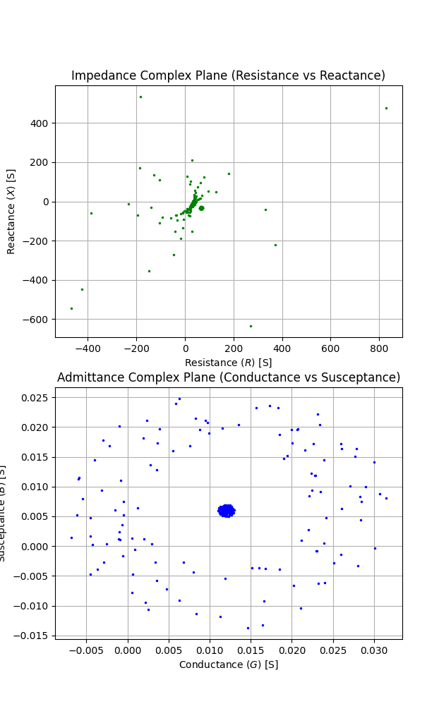
The admittance plot seemed beautiful to me 🤩.

(Initially I plotted the lines 😛 instead of dots, author told me to use dots only because lines make it messy and uninterpretable)

Now, the admittance plot looks like some pattern. I also confirmed with author after showing him the admittance plot, he said I am very close.

Now I needed to extract the flag from this plot. (the admittance one)

At this point I was sure that the flag is encoded in this plot only. But I am too tired to think anything new. I took a break scrolled reels, and came back with fresh mind.

I started observing the admittance plot carefully, I know that each points corresponds to a frequency value.

And the plot looks like very dense at center part with many points sourrounded by some scattered points.

What if I could iterate through all the admittances values (y11) for different frequencies and check wheter they lie in the center dense region or in the scattered region, depending on that I can assign 0 or 1 value to each admittance point.

It would form a binary string which I can convert to ascii to get the flag.

(Also it is evident from length of s11 or y11 which is 328 and 328/8 = 41 bytes, which is a good length for flag)

I used this code to extract flag:

seq = ""
for i, v in enumerate(y11):
    r = v.real
    im = v.imag
    print(f"Index: {i}, Conductance: {r}, Susceptance: {im}")

    # visually determined thresholds for dense region
    if (r > 0.010 and r < 0.015) and (im > 0.0025 and im < 0.0075):
        seq += "0"
    else:
        seq += "1"

print(seq)
print(len(seq))

This code gives me the a binary string which when converted to text dosen’t look like flag at all.

After struggling for few minutes, I got it…

The value 0x37 given in challenge description which I can’t use anywhere else, must be used here now.

I XORed each byte of binary string with 0x37 to get the final flag.


seq = ""
for i, v in enumerate(y11):
    r = v.real
    im = v.imag
    print(f"Index: {i}, Conductance: {r}, Susceptance: {im}")

    if (r > 0.010 and r < 0.015) and (im > 0.0025 and im < 0.0075):
        seq += "0"
    else:
        seq += "1"

print(seq)
print(len(seq))

binary_sequence = seq

flag = ""
for i in range(0, len(binary_sequence), 8):
    byte = binary_sequence[i:i+8]
    flag += chr(int(byte, 2)^0x37)
print(f"Decoded Flag: {flag}")

And this ladies and gentlemen this is how I got the flag -

Decoded Flag: flag{el3c7r1c4l_3ngin33ring_1s_wund3rb4r}

Ufff, tbh this was a long one and hectic too.

Anyways I was happy to solve it and got some nice points for my team. It was fun solving this challenge

Shoutout to author @Vx for this cool challenge.

Now I am a certified EE student ⚡😭

That’s all for now folks! Thanks for reading.

Final solution script - Click Here

Mizuhashi Simple Domain#

Mizuhashi Simple Domain